Explaining inflation and output volatility in chile: an empirical analysis of forty years

 

Explicando la volatilidad de la inflación y el producto en Chile: un análisis empírico de 40 años

 

Expliquant l'inflation et la volatilité du produit au Chili : une analyse empirique d'une quarantaine d'années

 

 

Juan de Dios Tena^I,*; César Salazar^II

^IUniversidad Carlos III, Departamento de Estadística, C/Madrid 126. 28903 Getafe (Madrid), España, e-mail: jtena@est-econ.uc3m.es and Universidad de Concepción, Departamento de Economía, Victoria 471, (Concepción), Chile. E-mail: juande@udec.cl
^IIUniversidad del Bío-Bío, Facultad de Ciencias Empresariales, Departamento de Economía y Finanzas, Av. Collao Nº 1202, Casilla 5-C, Concepción- Chile. E-mail: csalazar@ubiobio.cl

Replicated from Cuadernos de Economía, Bogotá, v.27 no.49, p. 259-279, July/Dec. 2008.

 

 

---

ABSTRACT 

This paper presents a data-oriented analysis of the effects of different kinds of economic shocks on Chilean output growth and inflation over the last 40 years. Two important results highlight the role of trade openness and countercyclical monetary policies to explain structural changes in the Chilean economy: (1) foreign shocks only explain 17% of the variability of output growth in the 1984-2006 period, whereas it used to account for 47.2% in 1966-1983; and (2) The relative importance of foreign shocks in explaining inflation volatility has become more important in the last twenty years. 

Key words: trade openness, volatility, inflation, output growth, structural VAR. JEL: E3, C3.

---

RESUMEN 

El artículo presenta un análisis empírico de los efectos de diferentes tipos de shocks económicos en el crecimiento del producto y la inflación chilena. Dos importantes resultados enfatizan el papel jugado por la apertura comercial y las políticas monetarias contracíclicas a la hora de explicar cambios estructurales en la economía chilena: (1) 17% de la variabilidad del producto entre 1984 y 2006 corresponde a shocks externos, mientras que entre 1966 y 1983 su impacto era de 47,2%; (2) en los últimos veinte años ha aumentado la importancia relativa de los shocks externos para explicar la volatilidad de la inflación. 

Palabras clave: apertura comercial, volatilidad, inflación, crecimiento, VAR estructural. JEL: E3, C3

---

RÉSUMÉ 

L'article présente une analyse empirique des effets de différents types de chocs économiques sur la croissance du produit et l'inflation au Chili. Deux résultats importants soulignent le papier joué par l'ouverture commerciale et les politiques monétaires contre-cycliques lorsqu'il s'agit d'expliquer les changements structuraux dans l'économie chilienne : (1) 17 % de la variabilité du produit entre 1984 et 2006 correspond aux chocs externes, tandis qu'entre 1966 et 1983 son impact était de 47,2 %; (2) dans les vingt dernières années il y a eu un accroissement de l'importance relative des chocs externes pour expliquer la volatilité de l'inflation. 

Mot clés : ouverture commerciale, volatilité, inflation, croissance, VAR structural. JEL : E3, C3.

---

 

 

This paper is a data-oriented analysis of the effect of a number of fundamental shocks in Chilean output volatility and inflation over the period 1966-2006. As far as we are aware, this is the first empirical analysis of this type of a developing country for such a long period. Although researchers have shown an increasing interest in explaining the factors that account for the sudden decline in output and inflation volatility to fundamental shocks in developed countries since the early 1980s¹, similar studies are still scarce for developing countries.

The literature shows a set of elements that determine the responsiveness of a small and open economy to foreign shocks. First, the evidence shows two views on the relationship between the openness of the economy and macroeconomic volatility. For example, Bejan (2004) and Easterly et al. (2001) found a positive correlation between volatility of product and trade liberalization. According to Forbes (2001), greater exposure to international markets facilitates the transmission of international crises through changes in levels of competitiveness, revenue and supply shocks. This vulnerability becomes more important in poor countries with greater specialization in production and less diversi­fication, countries with political instability, incomplete financial markets and weak institutions (see Calderon et al., 2005). On the other hand, according to Caballero (2002), vulnerability to shocks is a problem that can be seen from a financial perspective. In this regard, Bekaert et al. (2004) and Calderon et al (2005) show a negative relationship between volatility of output growth and financial integration. Finally, Eicher and Hull (2004) found empirical evidence that financial liberalization smoothes fluctuations of the product, but reduces the speed of convergence in the short term.

Secondly, there is consensus that a weak institutional framework could amplify the effects of external shocks. In this regard, Franken et al (2005) found evidence that the resilience of the Chilean economy to external shocks has increased in the 1990s thanks to anti-cyclical policies promoted by the government.

Some structural changes in the Chilean economy during second half of the period of interest can be mentioned considering the aspects discussed above. Since 1990, Chile has experienced a process of trade and financial liberalization on the basis of trade agreements and capital account openness. In the early 1990s, the Central Bank was given complete administrative and operational independence, adopting a regime based on an inflation target. At the end of the 1990s Chile adopted a structural surplus rule. Finally, in the second half of 1999, Chile abandoned the system of floating exchange rates, adopting a flexible exchange rate system.

An important difference between our work and this previous literature is that we use a structural vector autoregressive (VAR) approach to study the effect of different shocks. There are two important advantages in the use of this methodology in our particular context. Firstly, in our VAR system all the fundamental variables are endogenously determined. Thus, we can estimate the effect of unanticipated shocks on Chilean output and inflation. This overcomes some of the problems found in reduced form equations where movements in the explanatory variables fail to be exogenous as they can be anticipated by economic agents. Secondly, our VAR model for a single country allows for the estimation of the dynamic effect of different types of fundamental shocks over a long period of time. Panel data techniques, on the other hand, usually consider a set of heterogeneous countries for a short period of time and restrict slope parameters to be identical across countries. As discussed by Pesaran and Smith (1995), this can result in a highly misleading estimate of the parameters. 

The structure of this paper is as follows. The next section presents the data and tests for possible cointegration relationships. Section 3 discusses identification of VAR models and Section 4 analyses the responses of Chilean inflation and output growth to a number of fundamental shocks before and after 1983. In Section 5 we analyze the effect of different structural shocks on Chilean inflation and output using the approach in Lütkepohl and Reimers (1992). Some concluding remarks follow in Section 6.

 

PRESENTATION OF THE DATA AND COINTEGRATION ANALYSIS

We consider an approach similar to Dale and Haldane (1995) in the specification process. Thus, we test for possible cointegration among the series. When cointegration is found, the system is estimated at unrestricted levels; otherwise, it is estimated in differences.

The following endogenous variables are used in our analysis: the Brent price (B_t)²; the price of copper (C_t);  the Dow-Jones Index (D_t); the exchange rate expressed as the number of Chilean pesos for one dollar (Δe_t) in first differences; the (seasonally adjusted) U.S. GDP in first diffe­ren­ces (); the U.S. Consumer Price Index in annual differrences (); the federal funds rate (); the (seasonally adjusted) Chi­lean GDP in first differences (); and the Chilean Consumer Pri­ce Index in annual differences ().³  All the series are on a quar­terly basis and cover the period 1966:Q1-2006:Q3. Also, all the series, with the exception of , are in natural logarithm form. As typically occurs with VAR models, the specification is simply a statistical des­cription of the relationship among the variables in the analysis. However, we could justify the selection of the different variables by saying the Phillips Curve and the aggregate demand equation in a small economy like Chile should be augmented by including international variables.

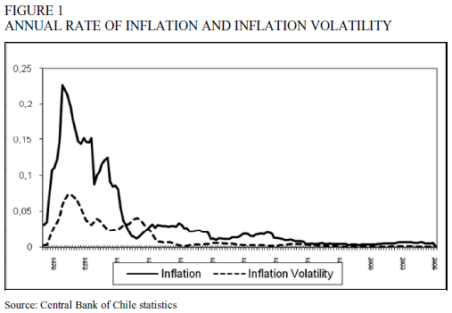
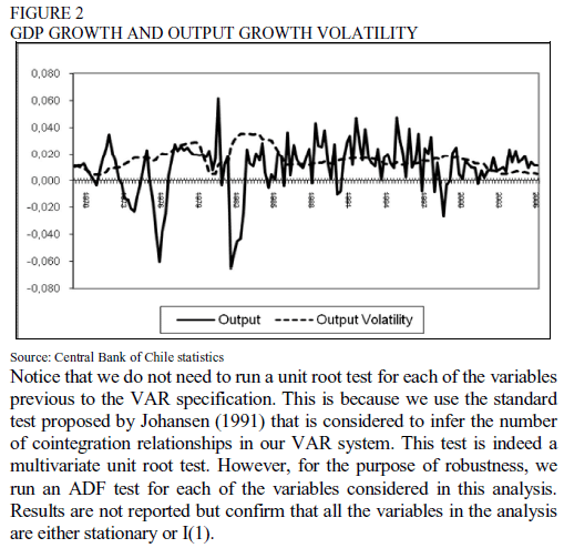
Figures of the series are not exhibited for the sake of brevity; however it is of interest for our analysis to observe the evolution of Chilean output growth and the annual rate of inflation. Figures 1 and 2 show the evolution of these two variables together with their volatility measures obtained from computing their rolling standard deviation with a window of four years; see Blanchard and Simon (2001) for a similar approach. A substantial reduction of inflation volatility through the sample period can be observed. The evidence of reduction in output volatility is not as compelling.

 

 

 

 

Notice that we do not need to run a unit root test for each of the variables previous to the VAR specification. This is because we use the standard test proposed by Johansen (1991) that is considered to infer the number of cointegration relationships in our VAR system. This test is indeed a multivariate unit root test. However, for the purpose of robustness, we run an ADF test for each of the variables considered in this analysis. Results are not reported but confirm that all the variables in the analysis are either stationary or I(1).

We consider a general specification with two lags to allow for short and long run adjustment in the data. This number of lags is also justified based on the Schwarz criterion.⁴ Also, following Juselius and Toro (2005), we start our analysis by considering a general specification of a vector equilibrium correction (VeqCM) model with intercept and trend in the cointegration equation but only intercept, and no trend, outside of the cointegration equation.

The trace test for cointegration indicates that the null hypothesis of at least 2 cointegration relationships can be rejected at the 1% level. It is of interest to show the equilibrium relationships among these variables over the last forty years. After testing for over-identifying restrictions, the 3 cointegration relationships can be expressed as:

 

	Δ4 PtCh = ΔytCh + Δ et	[1]
	itUS = 0.6* Δ4 PtUS	[2]
	ΔytUS = - Δ4 PtUS +0.005*(Bt + Δ 4 PtCh  + ΔDet ) %#150; 0.001*trend	[3]

 

The value of the likelihood ratio test for the over-identifying restrictions imposed in equations 1, 2, and 3 is χ²(ν) = 23.24(18). The p-value of the test is 0.18. Hence, over-identifying restrictions can be accepted at conventional levels. The cointegration relationships shown are also irreducible and the exclusion of any of the variables in expressions (1), (2) and (3) cannot be accepted using a likelihood ratio test at the 0.05 level.

A simple economic interpretation can be found for these equations. The first one relates inflation in Chile to output growth and the devaluation of the Chilean currency. The second one can be interpreted as a Taylor rule showing how the Fed rate reacts to inflationary pressures; and the third one indicates the negative effect of inflation on growth in the U.S.

In light of these results, we use an unrestricted VAR model to study the effects of different shocks in the Chilean economy. In order to allow the comparison of the effects of different shocks at different moments of time, we split our sample into two periods 1966:Q1-1983:Q4 and 1984:Q1-2006:Q3 and estimate two structural VAR systems.⁵

 

IDENTIFICATION OF THE STRUCTURAL MODEL

Now, we briefly discuss identification of our structural VAR models following the lines of Christiano et al. (2000). We estimate two reduced form models:

 

 

where  is a (nx1) vector of endogenous variables. In addition,  and  are polynomial matrices,  and  are (nx1) vectors of zero mean, serially uncorrelated disturbances while T^- represents all obser­vations up to 1983:Q4 and T⁺ all observations in 1984:Q1-2006:Q3.

These models do not allow for the computation of the dynamic response function of  (for k=1, 2) to the fundamental shocks in the economy. This is because the elements of a_t^k are, in general, contemporaneously correlated and it cannot be presumed that they solely correspond to a single economic shock. To deal with this issue, we consider two structural models defined by:

 

 

where , and  is a nth order matrix. The parameter matrices and errors in (4), (5), (6) and (7) are linked by,  and  with  being a (nx1) vector of orthogonal and standardized structural disturbances.

Once consistent estimators of the  in (4) and (5) are obtained, one can estimate Σ^k from the fitted residuals. All the information about the matrix  is contained in the relationship . Ho­wever,  has n² parameters while the symmetric matrix Σ^k, has at most [n(n+1)/2] distinct elements. The order condition specifies that at least [n(n-1)/2] restrictions are required to obtain a sufficient condition for identification. Additionally, the diagonal elements of  have to be positive.

The structural VAR system is identified by the recursiveness assumption including (in this order) the following endogenous variables in C_t, B_t and D_t. This amounts to assuming that commodity prices and financial variables react faster to economic information than output and price variables. It also means that Chilean economic variables react with one lag of delay to movements in the US variables. These are reasonable assumptions according to economic theory, while the main results are robust to changes in the identification assumptions. The recursiveness assumption implies that matrices  and  are lower triangular.

Our structural system is also used to decompose the forecast error variance of  into the proportions due to each shock; see for example Enders (2004), Chapter 5. This decomposition is very useful in our particular context because it tells us the proportion of the movement of the Chilean variables that is due to internal and external shocks.

 

ANALYSIS OF THE RESULTS

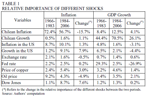
Table 1 shows the relative importance of different shocks to Chilean in­fla­­tion and output growth for the two periods considered in this analysis. At first glance, two important results can be mentioned from the obser­vation of this table. First, international shocks only account respectively for 41.7% and 17% of the inflation and output variance in the period 1984-2006. This is a striking result as one would expect that small open economies are very vulnerable to external shocks; see for example Forbes (2001) and Bejan (2004). Second, comparing the two periods, 1966-1983 and 1984-2006, it can be observed that the relative weight of foreign shocks on Chilean inflation has become more important in the most recent period, whereas the opposite can be said for Chilean output growth.

 

 

The first result can be explained by the precautionary policies under­taken by Chile to decrease exposure to short term capital flows and pressures toward excessive exchange rate appreciation. Concretely, Chile imposed reserve requirement on short term foreign indebtedness, crawling bands, and other instruments for reducing domestic vulnera­bility to capital flows; see Ffrench-Davis and Villar (2003) for a discussion of these policies and their effects.

Together with these precautionary measures, in the 1990s Chile perfor­med a unilateral liberalization strategy signing a number of trade agree­ments, among others with Canada and Mexico, and becoming a special associate member of Mercosur during this period. The price liberaliza­tion induced by these agreements can explain the increasing importance of international shocks to explain the Chilean inflation reaction.

Table 1 is also useful to analyze the importance of each individual shock for inflation and output growth. It can be observed that shocks in Chilean inflation and the price of copper are relatively important to explain output variation in the most recent period. However, Chilean inflation is mainly explained by shocks in US inflation and output growth. We show the effects together with the effect of shocks to copper and the Brent price in Figures 3 and 4⁶.

Notice that an unexpected shock in Chilean inflation only has a clear negative effect on growth in the period 1966-1983. In fact, this is an expected result as the 1970s was characterized by episodes of hyperinflation that affected output negatively. However, inflation is no longer a problem in the 1990s due to the independence of the Central Bank of Chile and the adoption of inflationary targets together with the aforementioned price liberalization. Additionally, impulses in the price of copper have a positive effect on output growth that last almost two years in the period 1984-2006.

Figures 3 and 4 also show that, as expected from the discussion in the previous section, Chilean inflation is more sensitive to the different shocks in 1966-1983 compared to 1984-2006. For example, consisten­tly with our insight, impulses in US growth increase Chilean inflation but the effect is stronger in 1966-1983. Also, unexpected US inflation generates an overreaction of Chilean inflation in 1966-1983 probably motivated by restrictions in the peso/dollar exchange rate that last for about 1 year. This effect is corrected during the next three years. Howe­ver, in the most recent period, Chilean inflation reacts positively and smoothly to shocks in US inflation.

Regarding the effect of the Brent price and copper on inflation, clearly their effect is stronger in the period 1966-1983 compared to the period 1984-2006. Also, they exhibit different signs in the two samples (negative for 1966-1983 and positive for 1984-2006). A plausible explanation for this is that commodity prices affect inflation by their transmission through cost and demand. In the period 1966-1983, industrial sectors are not important in the structure of the Chilean economy and all the transmission of an increase of commodity prices is through reduction in demand, whereas in the current period an increase in commodity prices raises the cost of many industries and therefore produces inflation in the short run. The effect of shocks to commodity prices on output is almost negligible in both periods.

To conclude this section it is also important to mention some the changes observed in the relative importance of the different individual shocks observed in Table 1. More specifically, comparing the two periods, shocks in the stock market index and US growth are becoming more important to explain Chilean inflation whereas oil shocks are losing importance. This is a reasonable result if we take into account the oil crises in the 1970s. Regarding Chilean growth, it is important to mention that, due to the measures in the 1990s to reduce the excessive exposure to short term capital flows, movements in Fed interest rates have reduced substantially its importance in the most recent period.

 

ESTIMATING THE EFFECT OF SHORT AND LONG-RUN SHOCKS

Models in the previous two sections consider nine different variables. This specification is used in an initial analysis to appraise the importance of the different types of shocks on Chilean inflation and output growth. However, from Table 1 it becomes clear that none of the shocks represents more than 10% of the variance of these two variables apart from US growth and inflation and the Fed funds rate. Therefore in this section we focus on studying the effect of shocks to Dy_t^US,  D₄ P_t^US, i_t^US on Chilean inflation and output. Also, in this analysis we consider the approach of Lütkepohl and Reimers (1992) instead of the approach of Christiano et al. (1999) as a robustness exercise. The main difference between these two methodologies lies in the fact that responses in Christiano et al. (1999) are based on an unrestricted VAR model whereas the approach by Lütkepohl and Reimers (1992) obtains responses from the MA representation of a VeqCM specification.

The variables included in the analysis are: the (seasonally adjusted) US GDP in first differences (Dy_t^US); the American Consumer Price Index in annual differences (D₄ P_t^US); the federal fund rate (i_t^US); the (seasonally adjus­ted) Chilean GDP in first differences (Dy_t^Ch); and the Chilean Con­su­mer Price Index in annual differences (D₄ P_t^Ch ). These are the varia­bles that explain at least 10% of inflation or output in any of the two periods.

We start by testing the number of cointegration relationships in a general specification that assumes constant and trend in the cointegration relationships and constant outside the cointegration equation (this corresponds to Case 4 in E-views software). Using the whole sample, the null hypothesis of at least zero, one and two cointegration relationships are rejected but the hypothesis of three cointegration relationships cannot be rejected at the 0.01 level. Therefore, VeqCM are specified with three cointegration relationships.

If some of the variables in expression (6) and (7) are cointegrated, they can be written as vector equilibrium correction (VeqCM) models.

 

 

Where  is a matrix whose rank is restricted to r (the number of cointegration relationships)

 

 

The structural forms associated to expressions (8) and (9) are

 

 

Now structural shocks are associated to reduced-form disturbances by .

Although the Wold representation does not exist for non-stationary cointegration processes, it is still possible to write the MA representation of Equations (8) and (9) using Johansen's version of Granger's Representation Theorem.

 

 

where  Ξ¹, Ξ², Ξ¹_j and Ξ²_j are coefficient matrices such that Ξ¹_j and Ξ²_j go to zero when j tends to infinity.  The terms Y₀¹ and Y₀² contain the initial values. Notice that Ξ  has rank n-r if the cointegration rank of the system is r. It represents the long-run forecast error impulse responses, whereas Ξ¹_j and Ξ²_j contain transitory effects for the two periods under analysis.

We still have to identify appropriate shocks for a meaningful impulse response analysis. If a_t^k is replaced by , the orthogonalized "short-run" impulse responses may be obtained as Ξⁱ_j(Aⁱ)^-1Bⁱ  in an analogous way to the stationary VAR case for i=1,2. The long-run effects of the structural shocks , are obtained as Ξⁱ_j(Aⁱ)^-1Bⁱ for i = 1,2.

The rank of this matrix is n-r and Aⁱ and B are nonsingular. Thus, the matrix ΞⁱBⁱ can have at most r columns of zero. Hence, there can be at most r shocks with transitory effects (zero long-run impact), and at least n^*=n-r . Due to the reduced rank of the matrix, each column of zeros stands for only n^* independent restrictions. Thus, if there are r transitory shocks, the corresponding zeros represent n^*r independent restrictions only. To identify the permanent shocks exactly [(n^*=n^*- 1)/2] additional restrictions are necessary. Similarly, for the transitory shocks we need [r(r-1)/2] additional contemporaneous restrictions to achieve identifica­tion; see King et al. (1991). Together, there are a total of  n^*r + [(n^*=n^*- 1)/2]+ [r(r-1)/2] restrictions and assuming A = I_n, we have just enough restrictions to identify B.

In our case, there are r=3 cointegration relations and two permanent shocks. The permanent shock is identified with one further assumption. For identification of the transitory shocks, three further restrictions are needed. We assume that US inflation and output growth in Chile and the US are not affected by the system variables in the long run. Additionally, because we need an additional restriction to identify the long run matrix, it is assumed that the Fed fund rate does not have a long run impact on Chilean inflation. For identification of the transitory shocks, three further restrictions are needed. Therefore, we assume that Chilean growth is not contemporaneously affected by the Fed funds rate and that US inflation is not contemporaneously affected by either Chilean inflation or Chilean growth. Although all these restrictions are subjective and cannot be tested, the main results remain under alternative identification assumptions.

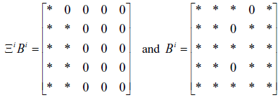
The restrictions imposed for variables (in this order)  i_t^US , Δ₄ P_t^Ch, Δ₄ P_t^US, Δy_t^US and  Δy_t^Ch are represented in the following framework

Notice that

 

 

where asterisks denote unrestricted elements.

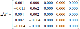
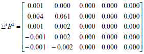
Results of this estimation for the two subsamples are shown below:

 

Before 1983

 

 

After 1983 

 

 

with the respective bootstrap t-values

 

 

The most important difference between the long run effects in the two periods is that the influence of Chilean output growth on Chilean inflation was negative (and significant) before 1983 and positive (and significant) after 1983.  A plausible explanation for this is that Chile suffered from hyperinflation in the seventies and this negatively correlated with output, while the relationship between Chilean inflation and growth after 1983 is more consistent with the expected sign of the Phillips curve.

Using this identification scheme, the response of Chilean growth and inflation to the different types of structural shocks is depicted in the following two figures (figure 5 and 6).

Consistent with the results in the previous section, the responses in these figures show that inflation is clearly less affected by all types of economic shocks in the period 1984-2006 compared to the 1966-1983 except for the effect of shocks to the Fed funds rate. In fact, this could be an indication that Chilean capital markets are less restricted, and therefore more affected by international interest rate movements, in the actual period. In the case of output growth, evidence about the different effects of shocks in the two periods under analysis is not as compelling, but still we can observe that most of the shocks have a bigger influence before 1983. 

 

CONCLUDING REMARKS

We present a data-oriented analysis of the effect of different kind of economic shocks on Chilean output growth and inflation over the last 40 years. The first notable result found in this study is that foreign shocks only explain 17% of the variability of output growth in the period 1984-2006 whereas it used to account for 47.2% of output variability in 1966-1983. Together with this effect, we found that, due to price liberalization and Chile's openness to international trade, the relative weight of foreign shocks to explain the Chilean inflation reaction becomes more important.           

In the most recent period shocks associated with inflation and growth in the US have not generated important reactions in Chilean inflation, in contrast with the observations from the period 1966-1983. This situation is explained by the implementation of monetary policy rules in the 1990s that work as a stabilizing macroeconomic instrument under a credible inflation targeting regime. Additionally, Chilean growth reaction is weaker in the period 1984-2006. The results suggest a major capacity of the Chilean economy to confront foreign shocks in the period 1984-2006. However, the evidence is much stronger for Chilean inflation.

The combined effect of these results is useful to explain why Chilean growth was almost immune to the tequila crisis in 1995. Moreover, the Asian and Russian crises in 1997 and 1998 respectively did not have the dramatic consequences observed in other developing countries.

An important lesson from our analysis is that Chile shows very specific features that are not shared with other Latin American countries. Therefore, this paper suggests that an empirical assessment of the importance of different policies for reducing the volatility of inflation and output growth should be based on models that do not impose slope parameters to be identical across countries.

 

BIBLIOGRAPHY

 1. Bejan, M. (2004). Trade Openness and Output Volatility, October, Mimeo, ITAM.

 2. Bekaert, G., H. Campbell, and C. Lundblad (2004). "Growth Volatility and Financial Liberalization", NBER Working Paper No. 10560.

 3. Blanchard, O. and Simon, J. (2001). "The Long and Large Decline in US Output Volatility", Brookings Papers on Economic Activity, 2001: 1.

 4. Caballero, R. J. (2002), "Coping with Chile's external vulnerability: a financial problem", Working Papers Central Bank of Chile 154, Central Bank of Chile.

 5. Calderón, C., Loayza, N. and Schmidt-Hebbel, Klaus (2005) "Does Openness Imply Greater Exposure? ", World Bank Policy Research Working Paper No. 3733.

 6. Christiano, L.J., Eichenbaum, M. and Evans, Ch. (1999). "Monetary shock: What we have learned and to what end" in Handbook of Macroeconomics, Volume A, Editors: John B. Taylor, Michael Woodford, North-Holland, 65-148.

 7. Dale, S. and Haldane, F. (1995). "Interest Rates and the Channels of Monetary Transmission: Some Sectoral Estimates", European Economic Review, 39: 1611-1626.

 8. Easterly, W., Islam, R. and Stiglitz, J.E. (2001). "Shaken and Stirred: Explaining Growth Volatility", Annual World Bank Conference on Development Economics, Ed. by B. Pleskovic and N. Stern.

 9. Eicher, T. and Hull, L. (2004). "Financial liberalization, openness and convergence" Journal of International Trade & Economic Development, 13 (4): 443-459.

 10. Enders, W. (2004). "Applied Econometric Time Series", New York: Wiley and Sons.                                                         

 11. Ffrench-Davis, R. and Villar, L. (2003). "The Capital Account and Real Macroeconomic Stabilization: Chile and Colombia", presented at the Seminar on Management of Volatility, Financial Liberalization and Growth in Emerging Economies, ECLAC Headquarters, Santiago.

 12. Forbes, K. (2001). "Are Trade Linkages Important Determinants of Country Vulnerability to Crisis? ", NBER Working Paper 8194, National Bureau of Economic Research.

 13. Franken, H. and Le Fort, G. and Parrado, E. (2005). "Business Cycle Dynamics and Shock Resilience in Chile," Working Papers Central Bank of Chile 331, Central Bank of Chile.

 14. Johansen, S. (1991). "Estimation and Hypothesis Testing of Cointegration Vectors in Gaussian Vector Autoregressive Models", Econometrica, 59: 1551-1580.

 15. Juselius, K. and Toro, J. (2005). "Monetary transmission mechanisms in Spain: The effect of monetization, financial deregulation, and the EMS", Journal of International Money and Finance, Elsevier, 24 (3): 509-531.

 16. Leduc, S. and Sill, K. (2003). "Monetary policy, oil shocks, and TFP: accounting for the decline in U.S. volatility", Working Papers 03-22, Federal Reserve Bank of Philadelphia.

 17. Lütkepohl, H. and Reimers, H.-E. (1992) "Impulse response analysis of cointegrated systems", Journal of Economic Dynamics and Control, 16: 53-68.

 18. King, R.G., Plosser, C.I., Stock, J.H. and Watson, M.W. (1991) "Stochastic trends and economic fluctuations", American Economic Review, 81: 819-840.

 19. Pesaran, M.H. and Smith, R.P. (1995), "Estimating long-run relationships from dynamic heterogeneous panels", Journal of Econometrics, 68: 79-113.

 20. Summers, P.M. (2005). "What caused the Great Moderation?: some cross-country evidence", Economic Review, Federal Reserve Bank of Kansas City, issue Q III, 5-32.

 21. Tena, J.D. and Giovannoni, F. (2005). "Market Concentration, Macroeconomic Uncertainty and Monetary Policy", University of Bristol Economics, Discussion Paper No 05/576.

 22. Tena, J.D., Sotoca, S., Jerez, M. and Carvallo, N. (2006). "A proposal to obtain a long quarterly GDP series", Latin American Journal of Economics, 43: 285-299.

 

 

Este artículo fue recibido el 30 de septiembre de 2007 y su publicación aprobada el 26 de junio de 2008.

 

 

¹ See Tena and Giovannoni (2005), Leduc and Sill, (2003) and Summers (2005) for some examples.
² There are many indicators for the price of oil. In the paper we use the Brent price as this is a very popular variable.
³ All these series were obtained from different sources. Specifically, the oil price was obtained from Dow Jones & Company, the U.S.GDP from U.S. Department of Commerce: Bureau of Economic Analysis, the Chilean Consumer Price Index from National Statistical Institute of Chile (ENI), the Chilean GDP from Tena et al. (2006) based on information provided by the Central Bank of Chile, and the price of copper, the Dow-Jones Index, the U.S. Consumer Price Index, the exchange rate and the federal funds rate from the Central Bank of Chile.
⁴ For example, the values of the Schwarz criterion of a model with two and three lags are respectively -39.65 and -38.22.
⁵ In some additional experiments not reported here we split the sample at 1979:Q4, 1980:Q4, 1981:Q4, 1982:Q4 and 1984:Q4. However, the main results of the papers were not altered in any of the experiments.
⁶ We do not show reactions to all possible shocks to save space but they can be obtained from the author upon request.  We are more explicit about the effect of different individual shocks in Section 5.